TUTORIAL: EXPLORATORY DATA ANALYSIS

INTRODUCTION

If you are familiar with data analysis then I’m certain that you fully relate to the above statement. After all, it would be pointless to play around with lots of data just for the love of it, sometimes not but you get the point.

Data is gold, and the more you have the better off you are. However, raw unprocessed data is of no use unless you manipulate and gain insights from it. Before embarking on say statistical modelling and visualization of your data, it is very important to first have an understanding of the data itself. Exploratory Data Analysis (EDA) aids in visualization, transformation, and generally cleaning or remodeling data before diving deep into information extraction.

There are no set rules to be followed when performing EDA. As a data preparation phase, one is allowed to decide what suits them best in order to gain an understanding of their data. However, there are two most important questions one should seek to answer while studying their data:

• Is there variation within my variables?
• Is there any correlation between my variables?

That being said, EDA involves the following checks among others:

• Descriptive Statistics - Gives a summarized understanding of the data, usually as measures of central tendency and variability.
  • Mean - Arithmetic average
  • Median - middle value
  • Mode - most frequent value
  • Standard Deviation - variation from the mean
  • Kurtosis -peakedness of the data distribution
  • Skewness - symmetry of the data distribution
• Groupings of data
• Missing values
• ANOVA: Analysis of variance
• Graphical visualization, not restricted to:
  • Histogram -frequency bar plots
  • Density estimation - an estimation if the frequency distribution based on sample data
  • Box plots - A visual representation of median, quantiles, symmetry and ourtliers
  • Scatter plots - a graphical display of variables plotted on the x and y axes.

In this post, we will perform EDA on a sample data set containing responses to a mobile banking survey in Kenya. If you would like to follow along with the same data, you can download it here.

DATA IMPORTATION

The code chunk below imports our data set into R.

#Loading Data into R  toc_depth: 2
mobileBanking.Df <- read.csv("J://Personalprojects//Blogsite//data//MobileBankinginKenya.csv", header = TRUE, stringsAsFactors = FALSE )
mobileBanking.Df <- mobileBanking.Df[,-1] #Remove the number column which is Irrelevant

1.0.0 Data Inspection

Once our sample data set is loaded, we check for features present. We first need to load all the libraries needed for data analysis and manipulation.

 #Load required packages or install if not present.----
load.libraries <- c('data.table','tidyverse','gridExtra', 'corrplot', 'GGally', 'ggplot2', 'e1071', 'dplyr')
install.lib <- load.libraries[!load.libraries %in% installed.packages()]

for(libs in install.lib) install.packages(libs, dependences = TRUE)

#Load libraries and flag TRUE
sapply(load.libraries, require, character = TRUE)

The function above takes in a list of required libraries, checks if they are already installed and installs them if not. It then loads all the packages one at a go.

1.1.0 Observing the data structure

dim(mobileBanking.Df)
## [1] 43 11

The data set has 43 rows with 11 Variables. We therefore explore the data types of each variable/column.

#Check Categorical VS Numeric Characters----
cat_vars <- names(mobileBanking.Df)[which(sapply(mobileBanking.Df, is.character))]
cat_vars
##  [1] "Gender"                       "Age.Range"                   
##  [3] "Have.Bak.Account"             "Bank.account.connected.to.MB"
##  [5] "MB.used.for"                  "Importance"                  
##  [7] "Benefit"                      "Bank.Visit"                  
##  [9] "MB.Safety"                    "Influence"                   
## [11] "Satisfaction"

numeric_vars <- names(mobileBanking.Df)[which(sapply(mobileBanking.Df, is.numeric))]
numeric_vars
## character(0)

To identify the data types, we can check for numeric and categorical variables present in the data. In our case, all the variables in our data set are categorical. We will therefore explore the data from a categorical approach rather than numeric. There exists different visualization methods for different data types. Now that we have established the general structure of the data, we can check for missing values, NAs.

#Checking data for any missing values
colSums(sapply(mobileBanking.Df, is.na))
##                       Gender                    Age.Range 
##                            0                            0 
##             Have.Bak.Account Bank.account.connected.to.MB 
##                            0                            0 
##                  MB.used.for                   Importance 
##                            0                            0 
##                      Benefit                   Bank.Visit 
##                            0                            0 
##                    MB.Safety                    Influence 
##                            0                            0 
##                 Satisfaction 
##                            0

We have no columns with missing values in our data. We can therefore proceed to analysis without worrying about missing values. In a case whereby there exists NA values, one can choose whether to replace the nulls with the most appropriate values or remove the rows with nulls from the data. This is important for later stages of analysis that include data modelling, like Machine Learning.

1.1.1 Data Summary

#Data Summary----
summary(mobileBanking.Df)
##     Gender           Age.Range         Have.Bak.Account  
##  Length:43          Length:43          Length:43         
##  Class :character   Class :character   Class :character  
##  Mode  :character   Mode  :character   Mode  :character  
##  Bank.account.connected.to.MB MB.used.for         Importance       
##  Length:43                    Length:43          Length:43         
##  Class :character             Class :character   Class :character  
##  Mode  :character             Mode  :character   Mode  :character  
##    Benefit           Bank.Visit         MB.Safety        
##  Length:43          Length:43          Length:43         
##  Class :character   Class :character   Class :character  
##  Mode  :character   Mode  :character   Mode  :character  
##   Influence         Satisfaction      
##  Length:43          Length:43         
##  Class :character   Class :character  
##  Mode  :character   Mode  :character

The base R Summary() function comes in handy at summarizing data. In our case, there is no statistical measures since all our variables are categorical. Note that the function also specifies the specific data types. There are more than enough ways to inspect data structures in R.

2.0.0 Getting Insights from the data

#Gender frequencies
#library(kableExtra)
table(mobileBanking.Df$Gender)
## 
## Female   Male 
##     20     23

#library(kableExtra)
# Cross classification counts for gender by Mobile banking safety opinion
table(mobileBanking.Df$Gender, mobileBanking.Df$MB.Safety)
##         
##          NotAtAll Somewhat Very
##   Female        3       11    6
##   Male          0       19    4

#Counts by gender, opinion and bank visits
table_ <- table(mobileBanking.Df$Gender, mobileBanking.Df$MB.Safety, mobileBanking.Df$Bank.Visit)
ftable(table_)
##                  FewTimesAyear OnceMonth
##                                         
## Female NotAtAll              3         0
##        Somewhat             11         0
##        Very                  5         1
## Male   NotAtAll              0         0
##        Somewhat             15         4
##        Very                  4         0

#library(kableExtra)
#Gender frequencies proportions
prop.table(table(mobileBanking.Df$Gender))
## 
##    Female      Male 
## 0.4651163 0.5348837

#Percentage idistribution for Gender by mobile banking safety
prop.table(table(mobileBanking.Df$Gender, mobileBanking.Df$MB.Safety))
##         
##            NotAtAll   Somewhat       Very
##   Female 0.06976744 0.25581395 0.13953488
##   Male   0.00000000 0.44186047 0.09302326

#Percentage by gender, opinion and bank visits, rounding off to 2 decimal places
table_ <- table(mobileBanking.Df$Gender, mobileBanking.Df$MB.Safety, mobileBanking.Df$Bank.Visit)
ftable(round(prop.table(table_),2))
##                  FewTimesAyear OnceMonth
##                                         
## Female NotAtAll           0.07      0.00
##        Somewhat           0.26      0.00
##        Very               0.12      0.02
## Male   NotAtAll           0.00      0.00
##        Somewhat           0.35      0.09
##        Very               0.09      0.00

# FREQUENCY MARGINALS
# row marginals - totals for each gender across mobile banking opinion
margin.table(table(mobileBanking.Df$Gender, mobileBanking.Df$MB.Safety), 1)
## 
## Female   Male 
##     20     23

# colum marginals -  totals for each gender across mobile banking opinion
margin.table(table(mobileBanking.Df$Gender, mobileBanking.Df$MB.Safety), 2)
## 
## NotAtAll Somewhat     Very 
##        3       30       10

# PERCENTAGE MARGINALS
# row marginals - row percentages across gender
prop.table(table(mobileBanking.Df$Gender, mobileBanking.Df$MB.Safety), margin = 1)
##         
##          NotAtAll Somewhat     Very
##   Female 0.150000 0.550000 0.300000
##   Male   0.000000 0.826087 0.173913

# colum marginals - column percentages acrossmobile banking opinion
prop.table(table(mobileBanking.Df$Gender, mobileBanking.Df$MB.Safety), margin = 2)
##         
##           NotAtAll  Somewhat      Very
##   Female 1.0000000 0.3666667 0.6000000
##   Male   0.0000000 0.6333333 0.4000000

#Loading Data into R  toc_depth: 2
mobileBanking.Df <- read.csv("J://Personalprojects//Blogsite//data//MobileBankinginKenya.csv", header = TRUE, stringsAsFactors = FALSE )
mobileBanking.Df <- mobileBanking.Df[,-1] #Remove the number column which is Irrelevant

#Check Categorical VS Numeric Characters----
cat_vars <- names(mobileBanking.Df)[which(sapply(mobileBanking.Df, is.character))]
numeric_vars <- names(mobileBanking.Df)[which(sapply(mobileBanking.Df, is.numeric))]


####Convert character to factors----
library(data.table)
setDT(mobileBanking.Df)[,(cat_vars) := lapply(.SD, as.factor), .SDcols = cat_vars]

mobileBanking.Df_cat <- mobileBanking.Df[,.SD, .SDcols = cat_vars]
    ##mobileBanking.Df_cont <- mobileBanking.Df[,.SD,.SDcols = numeric_vars]

#Functions for Plots---
library(ggplot2)
library(gridExtra)
plotHist <- function(data_in, i) {
  data <- data.frame(x=data_in[[i]])
  p <- ggplot(data=data, aes(x=factor(x))) + stat_count() + xlab(colnames(data_in)[i]) + theme_light() + 
    theme(axis.text.x = element_text(angle = 90, hjust =1))
  return (p)
}

doPlots <- function(data_in, fun, ii, ncol=3) {
  pp <- list()
  for (i in ii) {
    p <- fun(data_in=data_in, i=i)
    pp <- c(pp, list(p))
  }
  do.call("grid.arrange", c(pp, ncol=ncol))
}

plotDen <- function(data_in, i){
  data <- data.frame(x=data_in[[i]], SalePrice = data_in$SalePrice)
  p <- ggplot(data= data) + geom_line(aes(x = x), stat = 'density', size = 1,alpha = 1.0) +
    xlab(paste0((colnames(data_in)[i]), '\n', 'Skewness: ',round(skewness(data_in[[i]], na.rm = TRUE), 2))) + theme_light() 
  return(p)
  
}

Variable Distributions

#Plotting categorical values----
#Bar plots
doPlots(mobileBanking.Df_cat, fun = plotHist, ii = 1:4, ncol = 2)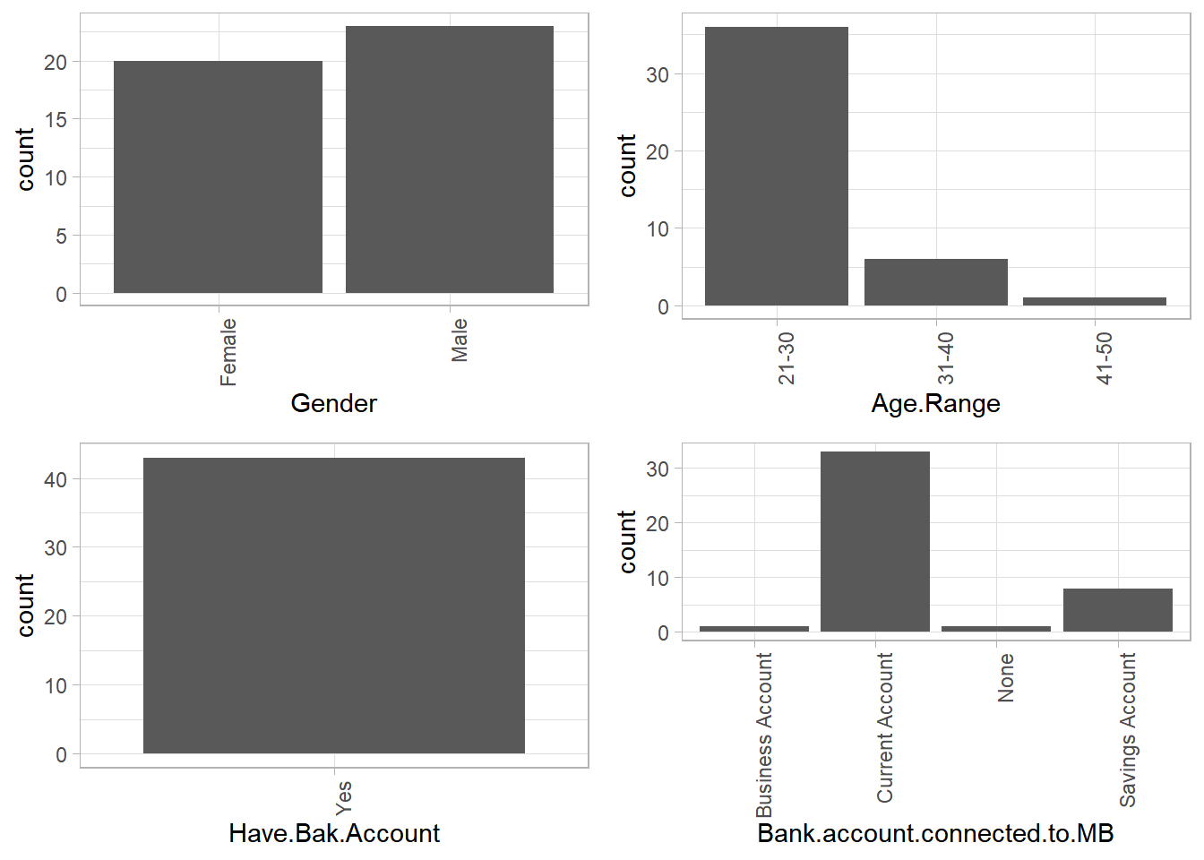

Gender

It can be seen that a larger number of respondents were male, this is however by a small margin. If we had a larger data set we could have more female respondents.

Age Range

A majority of respondents were younger guys between age 21-30, followed by the 31-40 age bracket. The least respondents were those above age 41. This could be probably because the older people chose not to participate in the survey as opposed to the younger ones, or that they somehow never got to opportunity to do so. A good example is the medium by which the survey was conducted, which the older people didn’t have.

Have Bank Account & Linked To Mobile Banking

All the respondents had bank accounts. A very small number had their business bank accounts linked to mobile banking. Majority had linked their current accounts probably due to the convenience that comes with mobile banking like frequent or timeless withdrawals.

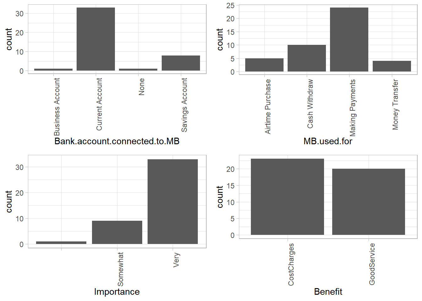
Uses Of Mobile Banking, Importance And Benefits

Most respondents use mobile banking services for making payments. This is followed by cash withdrawals. Airtime purchase and money transfer happen to be the least uses for the service. This could be because they are easily accessible needs unlike cash withdrawal and making payments in terms of mobility convenience.

Most respondents found mobile banking services very important, probably owing to the affordable cost charges and good service which could mean less usability issues when using the services.

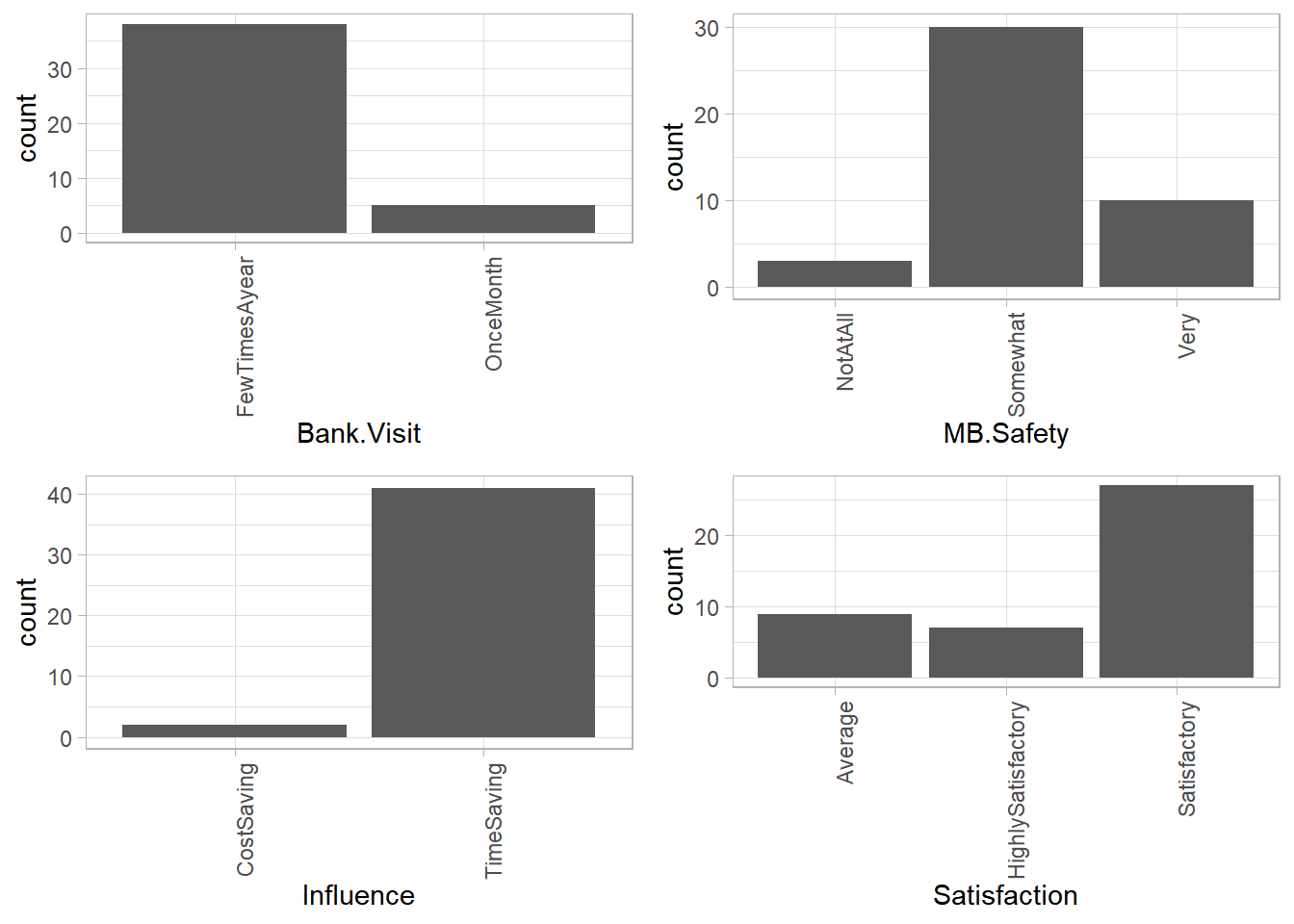
Bank Visits

We had most users who visit their banks a few times a year while the least do it once a month. This means that generally, fewer people visit the bank physically. This could be a major impact of mobile banking services.

Mobile Banking Safety, Influence And Satisfaction

Despite being majorly satisfied by the services, most respondents did not find mobile banking services very safe. It is also seen as time saving which is probably why we had very few bank visits in general.

Conclusion from variable distributions

It can be concluded that mobile banking is mainly preferred by younger people, a majority being of the male gender. However, the only benefit most users find from mobile banking seems to be the convenience it brings. Safety is still a major concern.

That’s basically it for exploratory data analysis. I made sure to cover the basics, meaning there’s still much to be added on to this; more visualizations, packages that simplify the whole process etc…This is to be continued. For a detailed documentation on the same, here’s Hadley Wickham’s R for Data Science book you can use as a reference point.